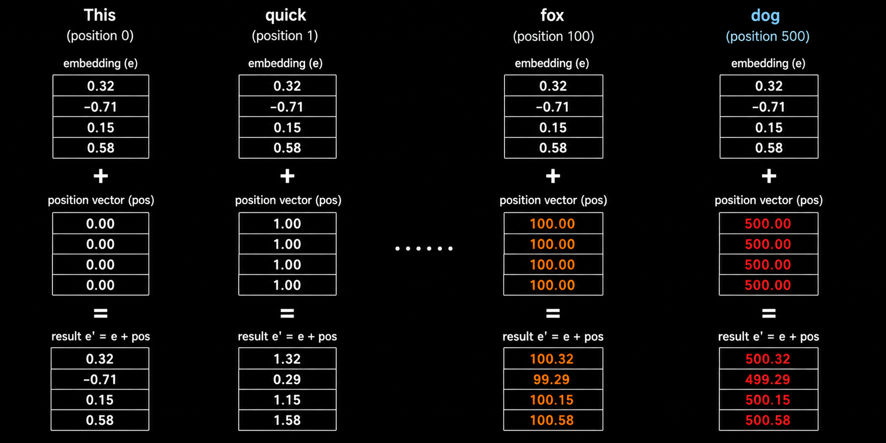
In Part 1, we explored three simple approaches to positional encoding. Direct integers, normalized values, and binary vectors.

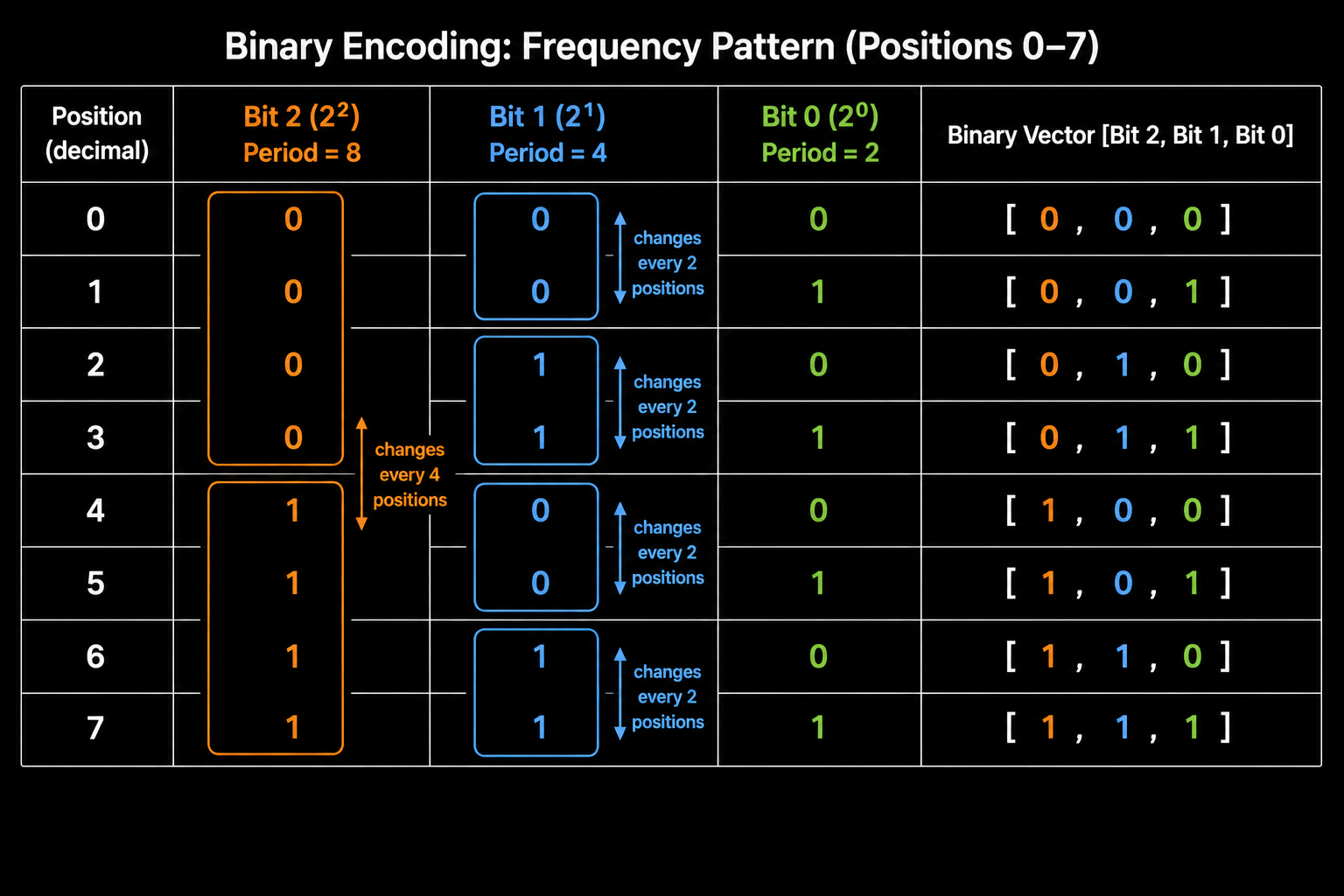
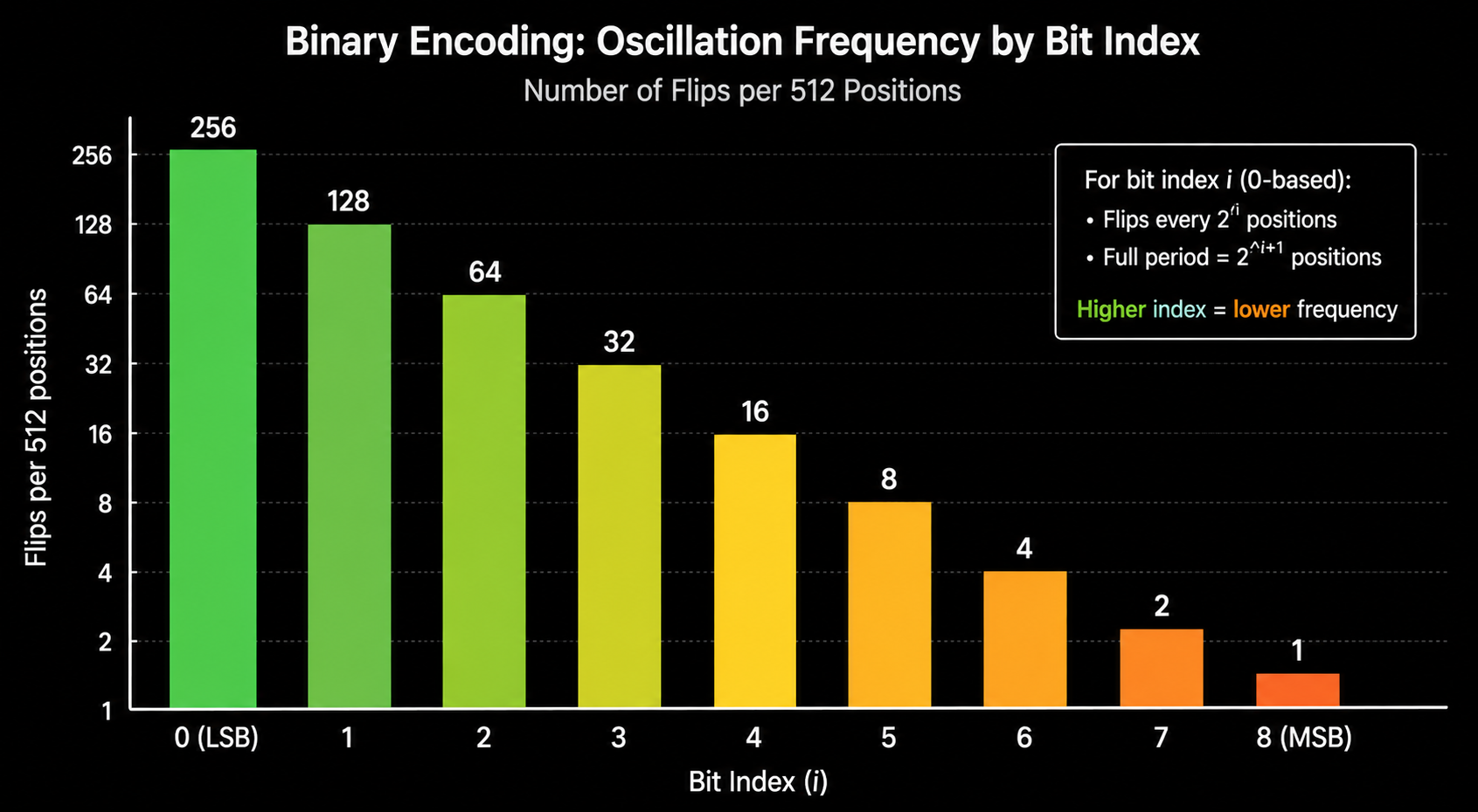
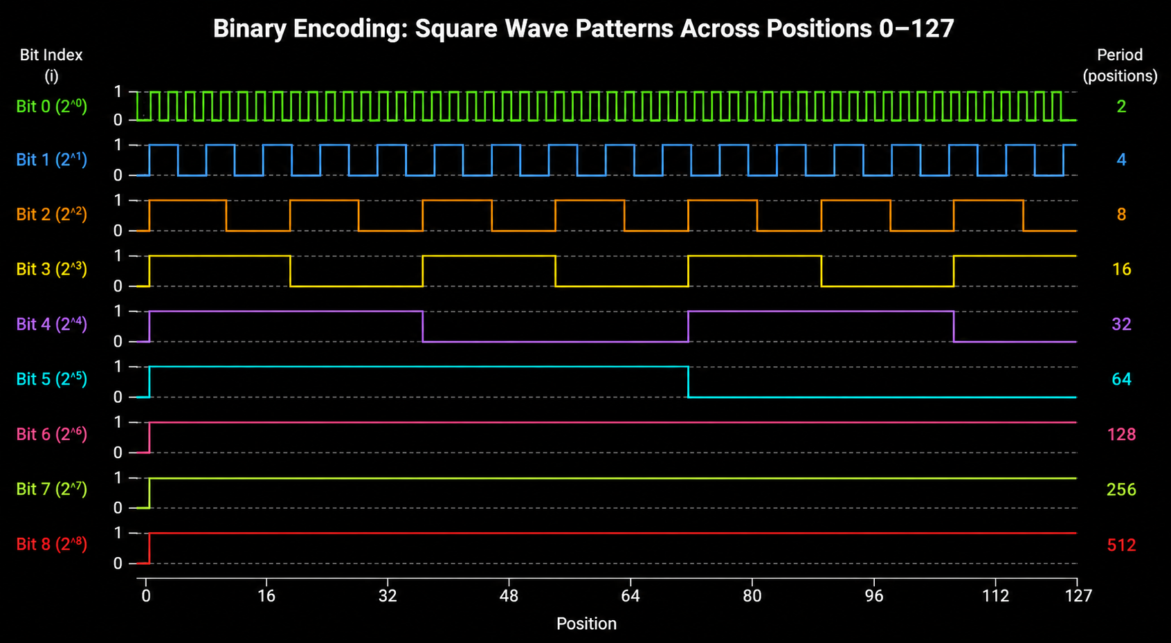
The most important lesson came from binary encoding. It revealed a multi frequency structure hidden inside position representations. Each bit oscillates at a different rate. Low bits flip rapidly, capturing fine grained position differences. High bits flip slowly, capturing coarse position in the sequence.

The structure was right. The problem was the shape. Square waves jump between 0 and 1 with no in between. Adjacent positions sometimes looked very different in vector space. Neural networks need smooth inputs to learn smooth functions.

Replace the square waves with smooth waves but keeping the multi frequency structure and making it continuous.

In this post, we will cover two approaches:

• Sinusoidal positional encoding, introduced in the original Transformer paper (Vaswani et al., 2017). It uses sine and cosine waves at geometrically spaced frequencies to give each position a unique, smooth, bounded vector.

• Rotary Position Embeddings (RoPE), introduced by Su et al. (2021). Instead of adding position to the embedding, it rotates the query and key vectors by their position. This makes relative position evident via the dot product naturally, with no learning required.

Sinusoidal encoding was a great step. But it has a structural limitation in how it mixes position with meaning. RoPE fixes that limitation, and is the method used in nearly every modern large language model today, including LLaMA, Mistral, Gemma, and Phi.

We will build both ideas step by step. Every formula will be derived from scratch. Every design choice will be motivated by a specific problem.

Let us start from exactly where Part 1 left off: the square waves of binary encoding and the two functions that make them smooth.

Idea 4: Sinusoidal Encoding

The Smoothest Periodic Function

The smoothest possible periodic function is the sine wave or cos wave.

A sine wave does not jump. It rises and falls continuously. Adjacent points on the wave are always close to each other in value. Two positions that are near each other will always produce sine values that are near each other.

Compare a square wave and a sine wave at the same frequency:

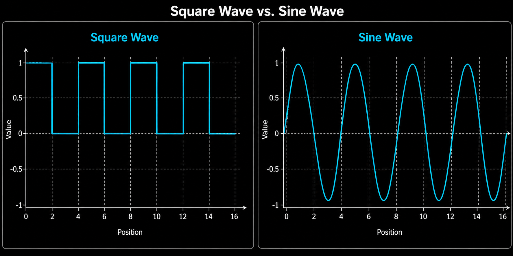
Both waves oscillate at the same rate. Both repeat at the same period. The difference is how they get from low to high. The square wave jumps. The sine wave moves smoothly.

Before we work out the formulas, it helps to actually see what these waves look like in motion.

The animation traces out sine waves at 3 frequencies (dim 1, dim 2, dim 3). As the position advances, the wave moves smoothly through space. There are no sudden jumps. There are no discrete flips. Every step from one position to the next is a continuous change.

Building a Multi Frequency Encoding

If we take inspiration from binary encoding, we want multiple sine waves stacked together. Each one oscillating at a different frequency.

For position $pos$ and dimension index $i$, the most natural starting point is:

Where $\omega_i$ is the frequency for dimension $i$.

Different dimensions get different frequencies. Some dimensions oscillate fast, like the LSB in binary. Others oscillate slow, like the MSB.

We now have to answer two questions:

1. How do we choose the frequencies $\omega_i$ for each dimension?
2. Is using only sine enough, or do we also need cosine?

The original Transformer paper answers both. Each one solves a specific problem.

Let us look at the frequency choice first.

Choosing the Frequencies

We need a range of frequencies. Some should be high, so the encoding can distinguish nearby positions sharply. Some should be low, so the encoding can carry information across long distances without repeating.

The paper uses this formula for the frequency of dimension pair $i$:

Where $d$ is the total dimensionality of the encoding.

Let us see what this gives us.

For dimension pair $i = 0$:

The wave oscillates rapidly. The value changes meaningfully with every position. This is the “fast bit” of the encoding.

For dimension pair $i = d/2$:

The wave oscillates extremely slowly. It barely changes over thousands of positions. This is the “slow bit” of the encoding.

Between these two extremes, the frequencies decrease smoothly on a geometric scale.

This is the same multi frequency structure we saw in binary encoding. Fast dimensions for fine grained position. Slow dimensions for coarse position. The difference is that every wave is smooth.

The general form:

Where $\omega$ is the frequency. Larger $\omega$ means the wave oscillates faster. Smaller $\omega$ means it oscillates slower.

To see this concretely, let us look at four sine waves with progressively lower frequencies. Consider x=pos and the number multiplied to the x (pos) be the frequency $\omega$

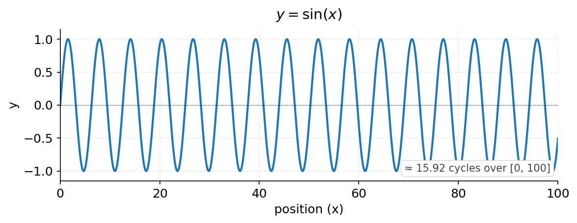
$\sin(x)$

This is the baseline. The wave completes one full cycle every $2\pi$ units. It oscillates rapidly.

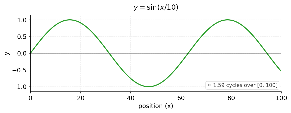
$\sin(x/10)$

Dividing the input by 10 stretches the wave horizontally by a factor of 10. The wave still does the same thing, but it takes 10 times longer to do each cycle. One full cycle now takes about 63 positions.

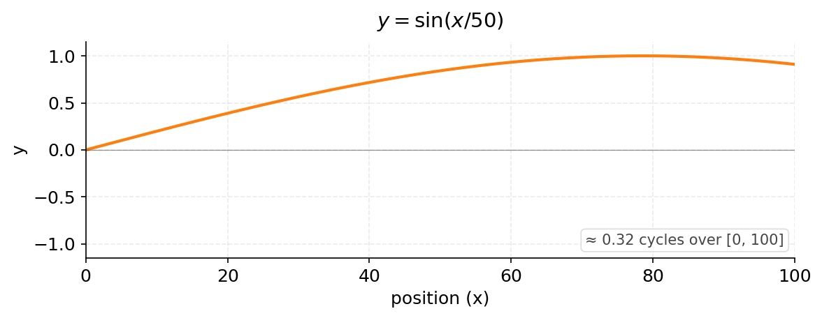
$\sin(x/50)$

Now the wave is very slow. Across 100 positions, we see only about 0.32 cycles. The wave is starting to look like a gentle curve rather than a rapid oscillation.

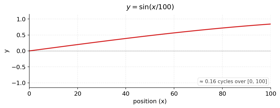
$\sin(x/100)$

At this frequency, we do not even complete one full cycle across 100 positions. The wave is nearly monotonic over the visible range. Adjacent positions look almost identical.

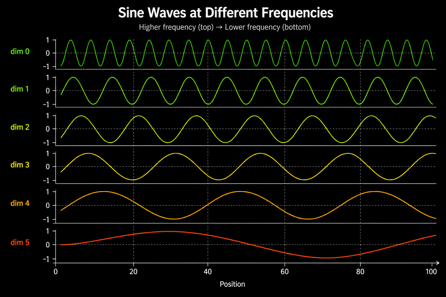
Stacking Them Together

If we stack these four waves on the same axis, we see the spectrum in one view.

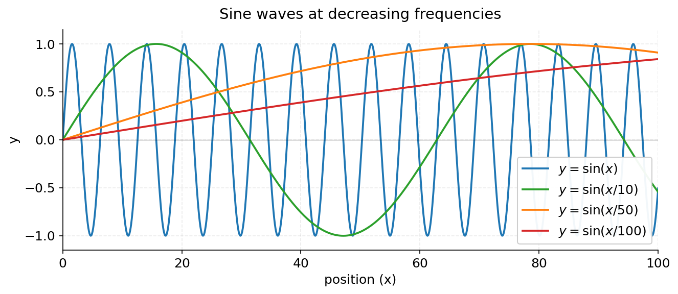
This is the same idea as binary encoding’s stack of square waves, but smooth. Fast waves capture fine grained position changes. Slow waves capture coarse, sequence wide position.

Each wave tells the model a different thing about where a token sits.

This gives us the visual intuition. The actual transformer formula controls this spectrum through the choice of base 10000. Let us see why.

Why 10000?

The number 10000 looks arbitrary. but its not.

It controls the range of frequencies. With a base of 10000, the slowest wave completes a full cycle every $2\pi \times 10000 \approx 62{,}832$ positions. This means within any reasonable sequence length, the slow dimensions never repeat. Every position gets a unique encoding.

let us plot the same encoding with three different base values: 100, 10000, and 100 million.

For each base, we will look at four different dimension indices to see how the wave behaves across positions 0 to 1000.

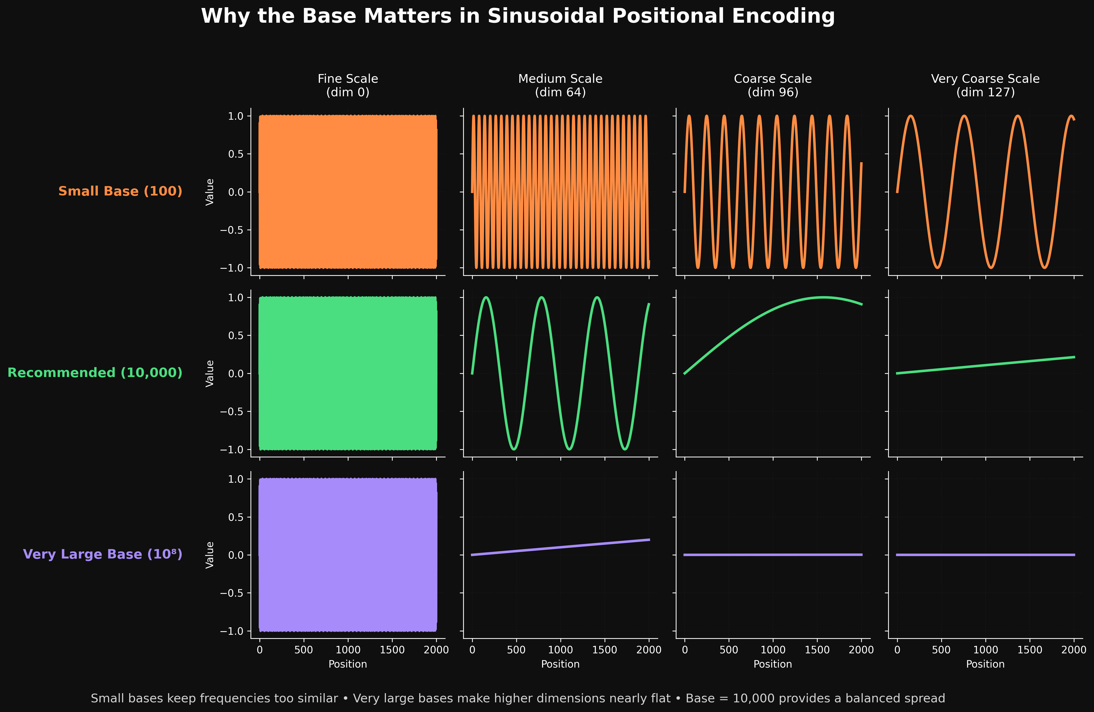
Each row shows one base value. Each column shows one dimension index. The top row uses base 100. The middle row uses base 10000. The bottom row uses base 100 million.

Base = 100 (top row)

Look at the four columns left to right.

• dim 0 oscillates rapidly. This is expected. Every base produces a fast wave at dim 0.

• dim 64 still oscillates a lot. Across 1000 positions, you see about good number of full cycles. The wave is far from slow.

• dim 96 also oscillates clearly. About good number of cycles across 1000 positions.

• dim 127 (the slowest dimension) still completes few full cycles in 1000 positions.

This is the problem with a small base. Even the slowest dimensions oscillate within the visible range. The waves repeat. Two positions far apart can produce identical encodings in every dimension simultaneously. The model loses its ability to tell distant positions apart.

A base of 100 spreads the frequency spectrum too narrowly. Everything moves too fast.

Base = 10000 (middle row)

This is the actual choice from the Transformer paper. Look at how the behavior changes.

• dim 0 still oscillates rapidly. The fast end of the spectrum is unchanged.

• dim 64 completes about 2 full cycles in 1000 positions. Slow enough to carry meaningful long range information, fast enough to differentiate positions.

• dim 96 does not even complete one cycle. The curve rises smoothly across the entire visible range. This dimension can distinguish between position 100 and position 800 because the values are different.

• dim 127 is nearly flat. The value barely changes from 0 to 0.1 across 1000 positions. This is the slowest end of the spectrum.

The spread is right. Fast dimensions stay fast. Slow dimensions actually get slow. Every position in a 1000 token sequence gets a unique vector across the full encoding.

Base = 100 million (bottom row)

Now look at what happens when the base is too large.

• dim 0 still oscillates rapidly. The fast end never changes with base.

• dim 64 is nearly a straight line. The wave has been stretched so far that it barely changes across 1000 positions.

• dim 96 is completely flat at zero.

• dim 127 is also completely flat at zero.

Most of the dimensions are useless. Their values are essentially the same across every position. They contribute no information about where a token is.

A base of 100 million spreads the frequency spectrum too widely. Almost the entire encoding is squeezed into the very slowest dimensions, which do nothing for typical sequence lengths.

The Problem

A smaller base, like 100, would cause the slow waves to repeat much sooner. Different positions would start getting identical encodings. The model would lose the ability to tell them apart.

A larger base, like a million, would spread the frequencies too thin. Most dimensions would oscillate too slowly to be useful.

The value 10000 was chosen to balance these two concerns. It is large enough to avoid repetition within typical context lengths, but not so large that the frequency spectrum becomes useless.

So Far, So Good

We now have a smooth multi frequency encoding. Every position gets a unique vector. The values are bounded between -1 and 1. The transitions between adjacent positions are continuous.

This is already a complete positional encoding. We could stop here and use just sine waves.

But the original Transformer paper does not stop here. Half of the dimensions use sine. The other half use cosine.

Why? What does cosine give us that sine alone does not?

Why Both Sine and Cosine?

We have a working positional encoding using only sine waves. Each position gets a vector. The values are bounded and smooth. The frequencies span from fast to slow.

So why does the original Transformer paper use sine for half the dimensions and cosine for the other half?

The formula assigns sine to even indexed dimensions and cosine to odd indexed dimensions:

Cosine looks redundant. It is just a shifted sine wave. So why include it?

The reason is a property called linear transformability.

Linear Transformability

We want the encoding to have a useful structure.

Given the encoding of one position, we want to reach the encoding of any other position using a simple linear operation.

If we know the encoding at position $pos$, we want to compute the encoding at position $pos + k$ by just multiplying with a matrix. And the same shift should always use the same matrix.

This is a strong property. If it holds, the model can reason about relative shifts using simple linear layers. This matters because $W_q$ and $W_k$ are exactly that, linear layers.

The Pair Representation

Take a single frequency $\theta$. Represent each position as a pair of values, one sine and one cosine:

Now, let us ask one question. Can we get from $PE(pos)$ to $PE(pos + k)$ using a fixed matrix?

We can transform using fixed matrix

Write down the encoding at position $pos + k$:

Expand each term using the angle addition formulas:

Look at the right hand side. Both new values are built only from $\sin(pos\,\theta)$ and $\cos(pos\,\theta)$. They are scaled by $\cos(k\theta)$ and $\sin(k\theta)$.

This is exactly a matrix multiplication:

Call this matrix $M_k$:

So we have:

The matrix $M_k$ depends only on the shift $k$. It does not depend on $pos$. The same shift always uses the same matrix.

This is the property we wanted.

Why Sine Alone Cannot Do This

Now try the same thing with only sine.

Suppose the encoding is just $\sin(pos\,\theta)$, a single value.

To get the encoding at $pos + k$, we need:

Look at the right hand side. It needs $\cos(pos\,\theta)$.

But a sine only encoding does not store $\cos(pos\,\theta)$. We only have $\sin(pos\,\theta)$. The term we need is missing.

There is no way to recover $\cos(pos\,\theta)$ from $\sin(pos\,\theta)$ using a linear operation. So the shift cannot be written as a fixed matrix.

The transformation is impossible with sine alone.

Why Cosine Is Needed

Cosine is the missing piece.

When we store both $\sin(pos\,\theta)$ and $\cos(pos\,\theta)$ together, both terms in the expansion are available. The matrix $M_k$ has everything it needs. The shift works.

This is why the encoding pairs sine and cosine at every frequency. It is not redundant. Cosine supplies the second component that makes the linear shift possible.

With both functions present, shifting a position becomes a rotation by the matrix $M_k$.

This rotation idea will come back in a much bigger way when we reach RoPE.

So, this relative information is learned by model implicitly not explicitly

How Sinusoidal Encoding Enters the Model

So far we have studied the positional encoding on its own. We derived its frequencies, its sine and cosine pairing, and its nice properties.

But there is a question we have not asked yet. How does this encoding actually get used inside the Transformer?

The answer creates a hidden problem. The clean properties we discussed do not fully establish once the encoding meets the rest of the model.

Two Properties, Two Places

Before we go further, let’s separate two things we have established.

The first is the dot product property. The dot product of two encodings gives $\cos(\theta(m - n))$, which depends only on relative position. This property matters inside the attention mechanism, where queries and keys are multiplied together.

The second is the linear shift property. A fixed matrix $M_k$ can shift an encoding from one position to another. This property matters for the linear layers in the model, such as $W_q$ and $W_k$.

These are two separate capabilities. They both need sine and cosine, but for different mathematical reasons.

Position Is Added to the Embedding

In the original Transformer, the positional encoding is added directly to the token embedding before anything else happens.

For a token at position $m$:

The embedding carries the meaning of the token. The encoding carries its position. We add them together into a single vector.

This combined vector is what flows into the attention mechanism. The model then computes queries and keys from it:

Each query and key now has two parts. A semantic part from the embedding, and a positional part from the encoding.

The Four Term Expansion

Now we compute the attention score. The score is the dot product of $Q_m$ and $K_n$.

Both $Q_m$ and $K_n$ have two parts. When we multiply two sums, every part of the first multiplies every part of the second. Two parts times two parts gives four terms.

Expanding gives four terms:

Let us read each term.

• Term 1 is purely semantic. It is the meaning of token $m$ against the meaning of token $n$. No position involved.

• Term 2 is a cross term. The meaning of token $m$ against the position of token $n$. Semantic mixed with position.

• Term 3 is the other cross term. The position of token $m$ against the meaning of token $n$. Position mixed with semantic.

• Term 4 is purely positional. The position of token $m$ against the position of token $n$. This is the term that contains $\cos(\theta(m - n))$, the clean relative position signal.

The relative position information we worked so hard to derive lives only in Term 4.

The Entanglement Problem

Here is the issue.

The model never sees Term 4 by itself. It sees the sum of all four terms. The clean relative position signal is buried inside a mixture.

Terms 2 and 3 are the troublemakers. They mix semantic content with positional content. They are noise sitting on top of the signal the model actually wants.

The model has to work through this mixture. There is no part of the architecture that isolates Term 4. The model must learn, on its own, how to make use of the relative position signal while ignoring the cross terms.

This creates a heavy burden on $W_q$ and $W_k$. These two matrices must do two jobs at once. They must project semantic meaning into a useful space. And they must preserve the positional structure so the relative position signal survives. Two competing goals, packed into one set of weights.

Absolute Versus Relative Position

There is a deeper issue here.

The encoding $PE_m$ stores absolute position. $PE_5$ is a fixed vector. It means position 5 and nothing else, no matter what sequence it appears in.

But what the model actually wants is relative position. It wants to know that two tokens are 9 apart, not that one is at position 5 and the other at position 14.

Relative position is not stored anywhere. It only appears as a byproduct, inside Term 4, after the dot product is computed. It is never represented directly.

So the model is given absolute positions and asked to figure out relative positions on its own. It can do this, but only by learning. There is no guarantee it learns it perfectly.

Position Is Fused With Meaning

There is one more limitation, and it is structural.

Once we compute $\text{embed}_m + PE_m$, the two parts are added into a single vector. They cannot be pulled apart again. Addition destroys the boundary between them.

Every layer after this point sees one fused vector. It cannot choose to look at only the meaning, or only the position. The two are tangled together for the rest of the network.

Sometimes the model only needs meaning. Sometimes it only needs position. But it cannot separate them. It is stuck with the mixture.

Summing Up the Limitations

Sinusoidal encoding is smooth, bounded, unique, and carries relative position inside its dot product. It was a real step forward.

But it has three weaknesses:

• Entanglement. Relative position is buried inside a four term mixture. Two cross terms add noise the model must learn to ignore.

• No direct relative position. The encoding stores absolute position. Relative position only appears as a byproduct of the dot product, never as an explicit representation.

• Fused representation. Position is added into the embedding and can never be separated. Every later layer is forced to handle the mixture.

All three problems share one root cause. Position is added to the embedding.

What if we did not add position at all? What if, instead of adding a positional vector, we applied position as an operation directly on the query and key?

This is the idea behind RoPE.

Idea 5: Rotary Position Embeddings (RoPE)

Sinusoidal encoding had three problems. All of them came from one decision: position was added to the embedding.

What if we never add position at all?

This is the idea behind RoPE, introduced by Su et al. in 2021. It is the positional encoding used in almost every modern large language model, including LLaMA, Mistral, Gemma, and Phi.

The Design Goal

In sinusoidal encoding, the attention score expanded into four terms. Only one of them carried clean relative position. The other two were noise that mixed meaning with position.

We want something better. We want the attention score to look like this:

One clean expression. The score should depend on the meaning of the two tokens and on their relative distance $m - n$. Nothing else. No cross terms. No entanglement.

The Key Insight

The problem with sinusoidal encoding was the order of operations.

We added position to the embedding first. Then we multiplied by $W_q$ and $W_k$. Because position was already mixed into the embedding, the multiplication produced cross terms.

RoPE flips the order. It does not touch the embedding. Instead, it lets $W_q$ and $W_k$ do their work first, producing the query and key. Then it applies position directly to those vectors.

In other words: apply position after the projection, not before.

Why This Helps

When position is applied after $W_q$ and $W_k$, those two matrices no longer have to deal with position at all. Their only job is to handle meaning. They project the token embedding into a query or key that captures semantic content. That is it.

Position becomes a separate, independent step. It is applied on top of the query and key as its own operation.

There are no longer two competing goals packed into $W_q$ and $W_k$. The projection handles meaning. The positional operation handles position. Each does one job.

Now the question becomes: what operation should we apply to the query and key to inject position?

The answer is rotation.

The Rotation Operation

Take a query vector. To keep things simple, let’s start with just two dimensions.

This query sits at position $m$. We pick a frequency $\theta$, the same kind of frequency we used in sinusoidal encoding.

To inject position, we rotate this 2D vector by an angle of $m\theta$. The rotation is done with a rotation matrix:

This uses the same sine and cosine values as sinusoidal encoding. But the operation is different. We are not adding anything. We are rotating the vector.

The position $m$ decides how much we rotate. A token at position 1 is rotated by $\theta$. A token at position 2 is rotated by $2\theta$. A token at position 100 is rotated by $100\theta$. The further along the sequence, the more the vector turns.

Writing Out the Rotation

Let us expand the matrix multiplication to see the new values directly.

The new query is a mix of the old components, weighted by sine and cosine of the rotation angle.

The length of the vector does not change. Rotation only turns the vector, it does not stretch or shrink it. The meaning carried by the magnitude stays intact. Only the direction shifts, and the amount of shift encodes the position.

We do the exact same thing to the key vector, using its position $n$:

Now both the query and the key have been rotated by their own positions.

The next question is what happens when we take the dot product of two rotated vectors.

Why Rotation Gives Pure Relative Position

We have rotated the query by its position and the key by its position. Now we take their dot product and see what comes out.

This is the heart of RoPE. The result is clean in a way sinusoidal encoding never was.

Setting Up the Angles

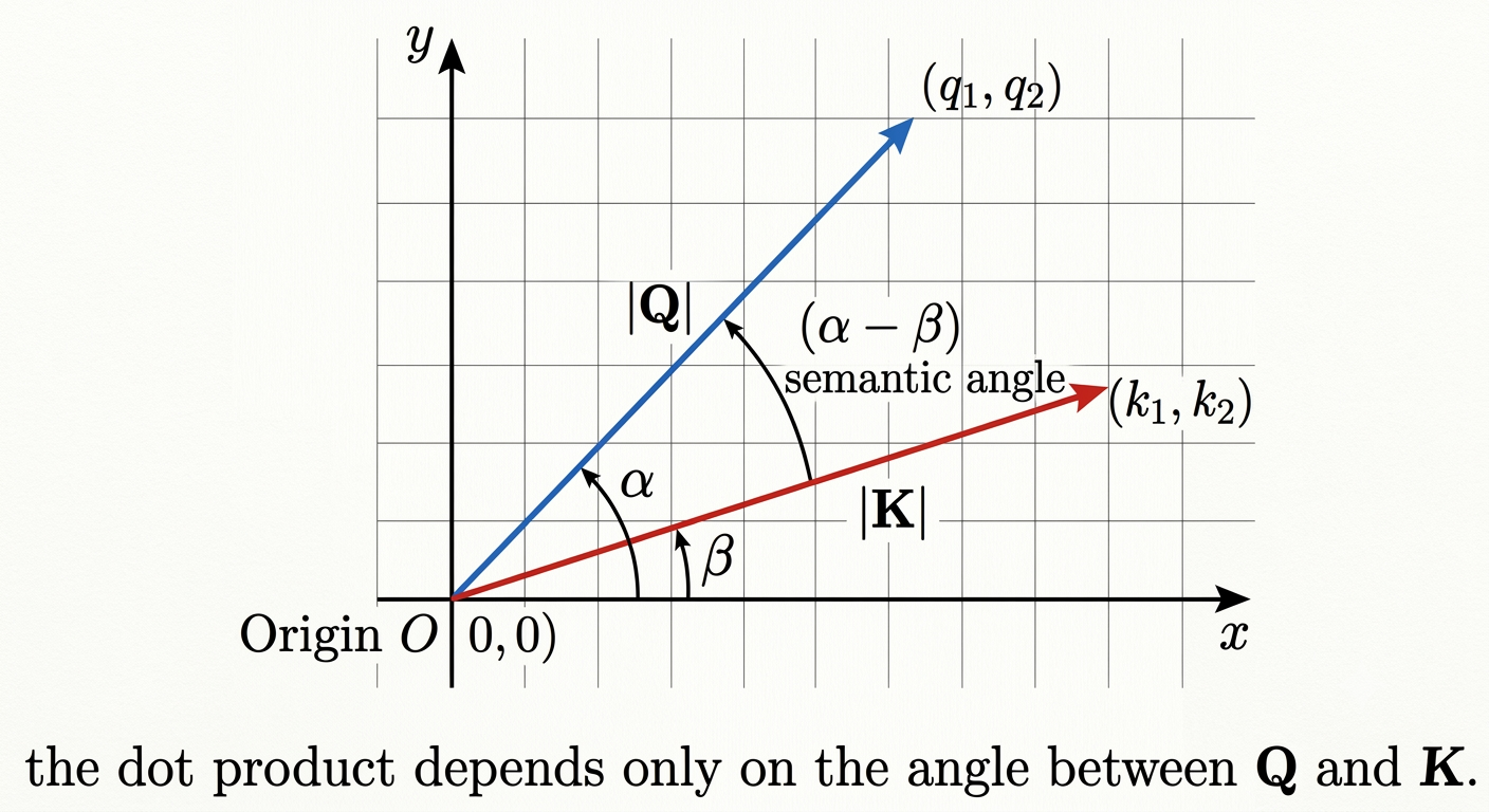
Every 2D vector has a direction, which we can describe with an angle.

Let the query $Q$ point in direction $\alpha$. This angle captures the semantic content of the query, the meaning that $W_q$ produced.

Let the key $K$ point in direction $\beta$. This angle captures the semantic content of the key.

Before any rotation, the dot product of two unit vectors depends on the angle between them:

The score depends on $\alpha - \beta$, the angle between the two directions. This is the semantic relationship between the query and the key.

Applying the Rotation

Now we rotate. The query is at position $m$, so we turn it by $m\theta$. The key is at position $n$, so we turn it by $n\theta$.

Rotation simply adds to the angle. After rotation:

Take the dot product of the rotated vectors. It depends on the angle between them, just like before:

Simplify the inside:

Look at this result carefully.

Reading the Result

There is one term. Just one. No four term expansion. No cross terms.

Inside the cosine there are two pieces:

• $(\alpha - \beta)$ is the semantic relationship. It is exactly the same angle that was there before rotation. It is untouched.

• $(m - n)\theta$ is the positional piece. It depends only on $m - n$, the relative distance between the two tokens.

The semantic part and the positional part sit side by side inside a single expression. The meaning is preserved. The position is relative. There is nothing to disentangle.

This is exactly the goal we set at the start. The attention score depends only on the semantics and on the relative distance $m - n$.

The Same Result Through Matrices

The angle argument is good, but let us confirm it with the matrices directly.

Write the rotated query as $R_m Q$ and the rotated key as $R_n K$, where $R_m$ and $R_n$ are rotation matrices. Their dot product is:

Rotation matrices have a special property. They are orthogonal, which means the transpose equals the inverse:

So the expression becomes:

Rotations combine by adding their angles. Rotating by $-m$ and then by $n$ is the same as rotating by $n - m$:

Putting it together:

The result depends only on $R_{n - m}$. The absolute positions $m$ and $n$ never appear on their own. Only their difference $n - m$ survives.

This is the same conclusion as the angle argument, now proven through the matrix algebra.

Does Rotation Corrupt Semantic Meaning?

There is a natural objection to all of this. Let us look at it carefully, because initially this is the doubt, I faced initially.

The Concern

The direction of $Q$ encodes the meaning of the token. That is what we said. The angle $\alpha$ carries semantic content.

Rotation changes the direction. After rotation, $Q$ points in a new direction $\alpha + m\theta$.

So if direction is meaning, and rotation changes direction, then rotation must change meaning. Rotation should corrupt the semantic content of the token.

This reasoning feels right. But it has a flaw.

Why the Reasoning Fails

The mistake is in the first step. Meaning in attention is not the direction of a single vector.

What the attention mechanism actually computes is the dot product between a query and a key. And the dot product depends on the angle between them, not on either direction alone:

The semantic relationship is $\alpha - \beta$. It is a relationship between two vectors, not a property of one.

Now look again at what rotation does:

The semantic relationship $(\alpha - \beta)$ is still inside the cosine. The rotation only added a positional piece next to it.

The meaning is preserved. It is combined with position, not removed or destroyed.

The Ideal Case

Consider two tokens at the same position, so $m = n$.

The positional piece becomes $(m - n)\theta = 0$. The dot product is:

This is exactly the original dot product, with no rotation effect at all.

Two tokens at the same position have their full semantic relationship, completely intact. Rotation changed nothing about the meaning.

Rotation Preserves Length

There is another way to see that rotation does not damage the vectors.

Rotation preserves length. A rotated vector has the same magnitude as the original. We can prove this directly.

The squared length of a rotated vector is:

Since rotation is orthogonal, $R^\top R = I$:

The length is unchanged. The magnitude of a query or key often carries learned information too, and rotation leaves it completely unchanged. Only the direction turns.

Where Do the Angles α and β Come From?

We have been talking about the query angle $\alpha$ and the key angle $\beta$. There is a common confusion about what these angles actually are. Let us clear it up.

Not the Embedding Angle

The angle $\alpha$ is not the angle of the token embedding.

Remember the order of operations. First the embedding goes through $W_q$. This produces the query. The angle $\alpha$ is the direction of that query, after the projection.

Same for the key. The angle $\beta$ is the direction of $K = W_k \cdot \text{embed}$, after projection by $W_k$.

These angles live in the query and key space. They are not angles in the original embedding space.

Why They Are Different Spaces

The projection matrix $W_q$ is rectangular. It might take a 768 dimensional embedding and produce a 64 dimensional query, one per attention head.

A rectangular matrix does not just rotate the vector. It reshapes it, reweights it, and drops it into a smaller space. The output direction has no simple relationship to the input direction.

So the angle of the embedding and the angle $\alpha$ of the query are not connected in any direct geometric way. The query angle is something new, created by the projection.

Then Why Does (α − β) Carry Meaning?

If $\alpha$ comes out of a projection, why does the angle $\alpha - \beta$ carry semantic meaning at all?

The answer is training.

$W_q$ and $W_k$ are not fixed. They are learned through gradient descent, together with the rest of the model. During training, the loss pushes these matrices to arrange the queries and keys in a useful way.

The arrangement that minimizes the loss is the one where:

• Tokens that should attend to each other get a small angle $(\alpha - \beta)$. A small angle gives a high cosine, which gives a high attention score.

• Tokens that should not attend get a large angle $(\alpha - \beta)$. A large angle gives a low cosine, which gives a low attention score.

So the semantic meaning inside $(\alpha - \beta)$ is not inherited from the embedding space. It is learned. Training shapes $W_q$ and $W_k$ until the angle between a query and a key reflects how strongly the two tokens should attend.

The query and key space is built by training to make $(\alpha - \beta)$ mean something. RoPE then rotates within that learned space.

Scaling to Full Dimensions

So far we worked with a 2D query. Real queries have many dimensions, often 64 or 128 per head. How does rotation work there?

The idea is simple. We split the vector into pairs and rotate each pair on its own.

Pairing the Dimensions

Take a query of dimension $d$. Split it into $d/2$ consecutive pairs:

Each pair is a little 2D vector. We rotate each one exactly the way we did before.

The key detail is that each pair gets its own frequency. Pair $i$ uses frequency:

This is the same frequency formula from sinusoidal encoding. Early pairs get high frequencies and rotate fast. Later pairs get low frequencies and rotate slowly.

Each pair is rotated independently. The first pair does not interact with the second pair. There is no mixing across pairs.

The Block Diagonal Matrix

If we write the full rotation as one big $d \times d$ matrix.

It is block diagonal. Along the diagonal sit $d/2$ small $2 \times 2$ rotation blocks, one per pair. Everywhere off the diagonal, the entries are zero.

Each block $R(m\theta_i)$ is the familiar $2 \times 2$ rotation matrix for pair $i$ at position $m$.

Does RoPE Hurt Attention Between Distant Tokens?

The attention score is $\cos((\alpha - \beta) + (m - n)\theta)$. The semantic part and the positional part sit together inside one cosine.

But look closely at those two parts. There is a tension between them.

The Tension

Imagine a paragraph that starts with “Naveen finished the report” and ends, many sentences later, with “He sent it to the team.” The word “He” refers back to “Naveen.” For the model to understand the sentence, the query for “He” must attend to the key for “Naveen.” Suppose these two words are 34 tokens apart.

The model wants them to attend. So the semantic angle $(\alpha - \beta)$ is small, which pushes the cosine up toward a high score.

But the positional part $(m - n)\theta$ is not zero. The tokens are far apart, so this term adds a real angle on top of the semantic one.

The two parts pull in different directions. The semantic angle wants the score high. The positional angle pushes the total angle up, which pulls the cosine down.

When the gap is large, the positional part can fight against the semantic signal. Does the position term quietly suppress attention between tokens that should be linked?

Why It Is Fine at Normal Distances

The answer is the frequency spectrum, and we already have the pieces.

The slow pairs have a tiny frequency. At a gap of 34, the extra angle they add is almost nothing:

That is a fifth of a degree. The positional part barely moves the cosine in the slow pairs.

And we saw that training pushes the long range signal exactly into those slow pairs. So the “He to Naveen” link lives where the positional cost is nearly zero. The semantic signal wins easily.

Multi head attention helps too. Different heads have their own $W_q$ and $W_k$. Some heads specialize in long range links and lean entirely on the slow pairs. The model has dedicated mechanism for exactly this case.

So at sentence and paragraph distances, the tension is real but harmless. The design routes long range signals to where position does not interfere.

Where It Genuinely Breaks

Now push the gap much further. Not 34 tokens. Try 32000 tokens.

Even the slow pairs have a small but nonzero frequency. Multiply it by a huge gap and the angle is no longer small:

Now the slow pair has rotated past 180 degrees. And past 180 degrees, the cosine is negative.

A negative cosine means the contribution is now opposite. The slow pair, which was supposed to carry the long range signal, is now pushing the score down. The model is being told to push these two tokens apart, even though they may be strongly related.

This is not the model being confused about distance. It is worse. The positional term has actively flipped and is working against the right answer.

This is a real, known limitation of RoPE. It is why so much research goes into extending RoPE to longer contexts.

What Happens When Rotation Passes 360 Degrees

The 180 degree problem points to a deeper issue. Rotation is periodic. Turn far enough and you come back to where you started. Let us look at what that means for position.

The Aliasing Condition

Cosine repeats every 360 degrees, or $2\pi$ radians. So two different gaps can produce the exact same cosine.

For a pair with frequency $\theta_i$, two gaps $g_1$ and $g_2$ give the same value when their difference completes a full number of turns:

for some whole number $k$. When this happens, the two gaps are indistinguishable in that pair. This is called aliasing.

Aliasing in Each Band

Fast pairs alias quickly. With frequency near 1, the gap repeats about every 6 tokens. Gap 1 and gap 7 look almost the same to a fast pair.

This may not seem good, but it is fine. Fast pairs are only meant for short range precision. They do their job locally and we never care them for long distances.

Slow pairs alias very slowly. With frequency near 0.0001, they do not repeat until about 62832 tokens. Within any normal context, they never alias.

So each band repeats at its own distance. Fast pairs repeat every few tokens. Slow pairs repeat only after tens of thousands.

Why the Spectrum Saves Us

Here is the beautiful part. A single pair aliases often. But the full set of pairs almost never aliases all at once.

For two gaps to be truly indistinguishable, they would have to alias in every pair at the same time. That means their difference would have to be a whole number of turns for the fast period, the medium period, and the slow period, all together.

So even though every pair aliases on its own, the combination of all pairs gives each gap a unique fingerprint.

The Real Danger Is Not Aliasing

Aliasing means the model confuses two distances. That is not good, but there is something worse, and we already saw it.

When a slow pair rotates past 180 degrees, its cosine turns negative. The model is not just confused now. It is actively pushed the wrong way. A pair that should support a long range link instead fights it.

This is the precise failure that appears at very long contexts. It is the structural reason that standard RoPE struggles past its trained context length, and the reason researchers built methods to go beyond it further.

Wrapping Up

Let us revise and see the whole journey.

We started with the simplest idea, adding the raw position number, and watched it fail on scale. We normalized it and it failed on consistency. We moved to binary vectors and found a beautiful multi frequency structure, but the jumps between positions broke smoothness.

Sinusoidal encoding fixed the smoothness. It gave every position a unique, bounded, smooth vector, and its dot product quietly carried relative position. But adding it to the embedding entangled position with meaning and forced the model to untangle four terms.

RoPE fixed the entanglement. By rotating the query and key instead of adding to them, it made the attention score depend cleanly on the semantic angle and the relative distance, with no cross terms. It preserved meaning, preserved length, and spread position across a spectrum of frequencies that the model learns to use, fast pairs for nearby tokens and slow pairs for distant ones.

But at very long distances the slow pairs eventually rotate too far, the cosine flips, and attention is pushed the wrong way. That limit is exactly what modern long context research works to mitigate the issue.

But for the sequence lengths that today’s models are trained on, RoPE is clean, efficient, and effective. That is why it used inside almost every modern large language model, from LLaMA to Mistral to Gemma to Phi.

References

1. Vaswani, A., Shazeer, N., Parmar, N., Uszkoreit, J., Jones, L., Gomez, A. N., Kaiser, L., Polosukhin, I. (2017). Attention Is All You Need. arXiv:1706.03762

2. Su, J., Lu, Y., Pan, S., Murtadha, A., Wen, B., Liu, Y. (2021). RoFormer: Enhanced Transformer with Rotary Position Embedding. arXiv:2104.09864

3. Biderman, S., Black, S., Foster, C., Gao, L., Hallahan, E., He, H., Wang, B., Wang, P. (2021). Rotary Embeddings: A Relative Revolution. EleutherAI Blog. blog.eleuther.ai/rotary-embeddings

4. Fleetwood. You could have designed state of the art positional encoding. fleetwood.dev/posts/you-could-have-designed-SOTA-positional-encoding

Language models process text as a sequence of tokens. While token embeddings can represent the meaning of individual words, they do not inherently represent where those words appear in the sequence.

For example, consider these two sentences:

The words are identical but their meanings are completely different because the order changed.

Positional encodings are techniques that allow Transformer models to incorporate information about token positions. They help the model distinguish between different token orders and reason about relationships between tokens across a sequence.

Over the years, several approaches have been proposed for representing positional information. Some are simple and intuitive, while others are mathematically elegant and widely used in modern large language models.

In this blog, we will build these ideas step by step, starting from the simplest possible approaches and gradually moving toward the methods used in modern Transformers.

We will cover:

• Direct position values
• Normalized position representations
• Binary position encodings
• Sinusoidal positional embeddings
• Rotary Position Embeddings (RoPE)

For each approach, we will understand the intuition behind it, see how it works mathematically, identify its limitations, and understand how those limitations naturally motivate the next idea.

By the end of this blog, you should have a solid understanding of how positional information is represented in Transformers, why different positional encoding methods were developed, and why modern language models rely heavily on techniques such as RoPE.

The Bag of Words Problem

Consider two sentences: “Dog bites man” and “Man bites dog.”

Same three words. Completely different meanings. Ideally language model must tell these apart.

A Transformer without positional encoding cannot distinguish between these two sentences. The math makes it impossible.

How Self Attention Computes Scores

Each token is first converted into an embedding vector. The model then projects these embeddings into queries and keys using learned weight matrices \(W_q\) and \(W_k\):

The attention score between token \(i\) and token \(j\) is their dot product:

Based on the above formula.

The score depends on the embedding of token \(i\) and the embedding of token \(j\). Nothing else. The positions related information for \(i\) and \(j\) do not appear anywhere in the formula.

Why Order Becomes Invisible

The word “dog” gets the same embedding vector whether it appears at position 1 or position 3. So the attention score between “dog” and “bites” is identical in both sentences.

In “Dog bites man”:

In “Man bites dog”:

Identical. This holds for every pair of tokens.

The full attention matrix for “Dog bites man” is identical to the full attention matrix for “Man bites dog.” Every value, every row, every column will be same.

Permutation Invariance

This property is called permutation invariance.

Shuffle the tokens in any order and the attention scores do not change. “Dog bites man” and “Man bites dog” and “Bites dog man” all produce the same attention pattern.

Embeddings are looked up by token identity, not by position. Position simply does not exist in the computation.

Without a mechanism to inject position, the Transformer is a bag of words model. It knows which words are present. It does not know where they are.

This is the problem that positional encodings exist to solve

Idea 1: Adding Raw Position Numbers

The Transformer needs to know where each token is. The simplest idea is to just tell it directly by adding its position.

Take the position of each token as an integer and add it to the embedding. Token at position 0 gets +0. Token at position 1 gets +1. Token at position 511 gets +511.

The Idea

Every token embedding is a vector of numbers, typically around the range of -1 to +1. The proposal is straightforward: take the position index and add it as a scalar to every dimension of the embedding vector.

where $i$ is the position of the token in the sequence.

For a sequence “Dog bites man”:

• Position 0: $e_{\text{dog}}’ = e_{\text{dog}} + 0$
• Position 1: $e_{\text{bites}}’ = e_{\text{bites}} + 1$
• Position 2: $e_{\text{man}}’ = e_{\text{man}} + 2$

Now “Dog bites man” and “Man bites dog” produce different embeddings because the same word gets a different number added depending on where it appears.

But we will face an issue with this approach.

The Scale Problem

Embedding values typically live in the range of -1 to +1 (But the range of values can vary relatively to higher number). These are small, carefully learned numbers that encode the meaning of each token.

Now consider what happens at position 500. We add 500 to every dimension of the embedding. A dimension that was 0.3 becomes 500.3. A dimension that was -0.7 becomes 499.3.

The positional number completely dominates the embedding. The semantic content of the token is over shadowed by a massive positional value. The model can barely see embedding of the token.

At position 0, the embedding is untouched. At position 500, the embedding is almost entirely overwritten by the position value. Tokens near the beginning of a sequence and tokens near the end, live in completely different numerical ranges, not only because they mean different things, but also because of where they appear.

No Upper Bound

This approach has no fixed range. The position value grows without limit as the sequence gets longer.

A model trained on sequences of length 512 has seen position values from 0 to 511 . At inference time, if the input has 1024 tokens, the model suddenly sees position values up to 1023. It has never encountered numbers this large during training.

This is an out of distribution problem. The model has no way to generalize to positions it has never seen.

Inconsistent Distance

The absolute difference between position 1 and position 2 is 1. The absolute difference between position 500 and position 501 is also 1.

But relative to the position values themselves, these gaps are very different.

The model cannot learn a consistent notion of “subsequent positions” because the same gap of absolute positional difference of 1 looks completely different depending on where in the sequence it occurs.

Three issues make raw integer positions unusable:

• Scale mismatch. Large position values dominate out the semantic content of embeddings. A token’s meaning becomes invisible behind its position number.
• No upper bound. Position values grow without limit. The model cannot generalize to sequence lengths it has not seen during training.
• Inconsistent distances. The same gap between two positions looks different depending on absolute position. The model cannot learn a uniform sense of distance.

The position values are unbounded and live on a completely different scale than the embeddings.

What if we fix the scale problem by forcing all position values into a fixed range?.

Idea 2: Normalized Positions

Raw integer positions failed because the values were too large. They overwhelmed the embeddings and had no upper bound.

Instead can we just: squeeze all position values into the range [0, 1].

The Idea

Divide each position by the length of the sequence minus one.

where $L$ is the total number of tokens in the sequence.

For a sequence of length 512:

• Position 0 → 0.0
• Position 255 → 0.5
• Position 511 → 1.0

Every position now maps to a value between 0 and 1. No matter how long the sequence is, the values never exceed 1. They sit comfortably in the same range as the embedding values.

The scale problem is gone. The model no longer has to deal with position values like 500 drowning out embedding values like 0.3.

So this works?

The Spacing Problem

Consider two sequences of different lengths.

A short sequence with 10 tokens:

The spacing between consecutive positions is 0.11.

A long sequence with 1000 tokens:

The spacing between consecutive positions is 0.001.

The gap between adjacent tokens is 100 times smaller in the long sequence than in the short sequence. Two tokens that are “one step apart” look very different to the model depending on sequence length.

Same Position, Different Values

The same position index maps to completely different values depending on the sequence length.

Position 5 in a 10 token sequence:

Position 5 in a 1000 token sequence:

The fifth token gets the value 0.556 in one case and 0.005 in the other. These are not even close.

The model cannot learn what “position 5” means because the value it receives changes with every input. A model trained mostly on short sequences will associate 0.5 with the middle of a sentence. When it sees a long sequence where 0.5 maps to position 500, the learned association breaks.

Why This Is Fundamental

The root cause is that this scheme is relative to sequence length. It does not encode absolute position. It encodes “how far through the sequence are we.”

Position 0 always means “beginning.” Position 1.0 always means “end.” But everything in between shifts depending on $L$.

This creates two failures:

• No consistent position identity. The same position index produces different values for different sequence lengths. The model cannot learn a stable representation for any position.
• No consistent spacing. The distance between consecutive positions depends on $L$. The model cannot learn a uniform notion of “adjacent tokens” because the numerical gap changes per sequence.

What We Need Instead

Both attempts so far used a single number to represent each position. The first attempt used numbers that were too large. The second attempt used numbers that changed meaning depending on context length.

What if instead of a single number, we represented each position as a vector? And what if that vector used a fixed, length independent pattern that gave every position a unique and consistent representation?

This is exactly what binary encoding do.

Idea 3: Binary Encoding

Both previous approaches used a single number to represent each position. That single number was either too large or too unstable across sequence lengths.

A different idea: represent each position as a vector of bits.

Positions as Binary Vectors

Every integer can be written in binary. We can use this binary representation directly as a position encoding vector.

For a 9 bit encoding:

Each position gets a unique vector of 0s and 1s. The dimensionality of the vector is $\lceil \log_2(L) \rceil$, where $L$ is the maximum sequence length. For a sequence of up to 512 tokens, we need 9 bits.

What Binary Encoding Gets Right

This approach fixes every problem from the previous two attempts.

Bounded values. Every entry in the vector is either 0 or 1. No position value ever exceeds 1. There is no risk of drowning out the embedding.

Unique per position. Every integer has a distinct binary representation. No two positions share the same vector. Position 5 is always [0, 0, 0, 0, 0, 0, 1, 0, 1], regardless of how long the sequence is.

Length independent. Unlike normalized positions, the encoding of position 5 does not change when the sequence length changes. Position 5 is the same vector whether the sequence has 10 tokens or 10,000 tokens.

Fixed dimensionality. The encoding uses $\lceil \log_2(L) \rceil$ dimensions. This grows very slowly. 10 bits can handle sequences up to 1024. 20 bits can handle sequences up to 1,048,576.

But something interesting is hidden in how these bits change across positions. Before we look at the problems, let us first look at the structure.

The Frequency Pattern in Binary

The binary representations for positions 0 through 7 is as below and if we look at each bit column separately.

Now read each column from top to bottom.

Bit 0 (the rightmost, least significant bit) flips every single position: 0, 1, 0, 1, 0, 1, 0, 1. It completes a full cycle every 2 positions.

Bit 1 flips every 2 positions: 0, 0, 1, 1, 0, 0, 1, 1. It completes a full cycle every 4 positions.

Bit 2 flips every 4 positions: 0, 0, 0, 0, 1, 1, 1, 1. It completes a full cycle every 8 positions.

The frequency of that wave depends on which bit position it is.

LSB vs MSB: Fast Bits and Slow Bits

This pattern generalizes to any number of bits. For bit position $i$ (counting from the right, starting at 0):

The least significant bit (LSB, rightmost, $i = 0$) oscillates the fastest. It flips at every single position. It has a period of 2.

The most significant bit (MSB, leftmost, $i = d-1$) oscillates the slowest. For a 9 bit encoding, it flips every 256 positions. It has a period of 512.

Bits on the right change rapidly. Bits on the left change slowly. Each bit position captures positional information at a different scale.

Visualizing the Square Waves

If you plot the value of each bit across all positions, you see a series of square waves stacked on top of each other. Each wave has exactly half the frequency of the one below it.

This is a multi frequency encoding. The lowest bit gives fine grained position information (is this an even or odd position?). The highest bit gives coarse position information (are we in the first half or second half of the sequence?).

This multi frequency structure is the most important observation about binary encoding. It will directly motivate sinusoidal positional encoding in the next subsequent blog.

The Discontinuity Problem

Despite this awesome frequency structure, binary encoding has a flaw.

Look at positions 3 and 4:

• Position 3: [0, 1, 1]
• Position 4: [1, 0, 0]

These two positions are adjacent. They are one step apart. But their binary vectors differ in all three bits. The distance between them in vector space is large.

Now look at positions 2 and 3:

• Position 2: [0, 1, 0]
• Position 3: [0, 1, 1]

Also adjacent. Also one step apart. But only one bit differs. The distance between them is small.

Adjacent positions have wildly inconsistent distances in the encoding space. The transition from 3 to 4 is a large jump. The transition from 2 to 3 is a tiny step. There is no smooth relationship between position and encoding.

This happens because binary numbers carry over. When all lower bits are 1, the next increment flips them all to 0 and flips the next higher bit to 1. These carry overs cause sudden large changes in the vector for what should be a small step in position.

Why Discontinuity Matters

Neural networks learn smooth functions. They work best when small changes in input produce small changes in output. If two positions are close together, their encodings should also be close together.

Binary encoding violates this. The model cannot learn a smooth notion of “nearby positions” because the encoding jumps unpredictably between adjacent positions.

What We Keep, What We Fix

Binary encoding gave us two valuable ideas:

• Multi frequency structure. Different bits capture position at different scales. Fast bits for fine detail, slow bits for coarse structure.
• Vector representation. Each position is a vector, not a single number.

But it also has one critical issue:

• Discrete jumps. The square wave transitions between 0 and 1 are discontinuous. Adjacent positions can have very different encodings.

The fix is can be simple. Replace the square waves with smooth waves. Replace the discrete 0/1 flips with continuous sine and cosine functions.

Keep the multi frequency structure. Make it smooth.

This is exactly what sinusoidal positional encoding does.Lets discuss about this in subsequent next blog!

Part 2 of this series covers sinusoidal positional encoding and Rotary Position Embeddings (RoPE) the method used in nearly every modern large language model including LLaMA, Mistral, and Gemma.

References

1. Vaswani, A., Shazeer, N., Parmar, N., Uszkoreit, J., Jones, L., Gomez, A. N., Kaiser, L., Polosukhin, I. (2017). Attention Is All You Need. arXiv:1706.03762

2. Su, J., Lu, Y., Pan, S., Murtadha, A., Wen, B., Liu, Y. (2021). RoFormer: Enhanced Transformer with Rotary Position Embedding. arXiv:2104.09864

3. Biderman, S., Black, S., Foster, C., Gao, L., Hallahan, E., He, H., Wang, B., Wang, P. (2021). Rotary Embeddings: A Relative Revolution. EleutherAI Blog. blog.eleuther.ai/rotary-embeddings

4. Fleetwood. You could have designed state of the art positional encoding. fleetwood.dev/posts/you-could-have-designed-SOTA-positional-encoding