Positional Encoding Explained: From Position to Binary Encoding (Part 1)
Introduction
Language models process text as a sequence of tokens. While token embeddings can represent the meaning of individual words, they do not inherently represent where those words appear in the sequence.
For example, consider these two sentences:
The words are identical but their meanings are completely different because the order changed.
Positional encodings are techniques that allow Transformer models to incorporate information about token positions. They help the model distinguish between different token orders and reason about relationships between tokens across a sequence.
Over the years, several approaches have been proposed for representing positional information. Some are simple and intuitive, while others are mathematically elegant and widely used in modern large language models.
In this blog, we will build these ideas step by step, starting from the simplest possible approaches and gradually moving toward the methods used in modern Transformers.
We will cover:
- Direct position values
- Normalized position representations
- Binary position encodings
- Sinusoidal positional embeddings
- Rotary Position Embeddings (RoPE)
For each approach, we will understand the intuition behind it, see how it works mathematically, identify its limitations, and understand how those limitations naturally motivate the next idea.
By the end of this blog, you should have a solid understanding of how positional information is represented in Transformers, why different positional encoding methods were developed, and why modern language models rely heavily on techniques such as RoPE.
The Bag of Words Problem
Consider two sentences: “Dog bites man” and “Man bites dog.”
Same three words. Completely different meanings. Ideally language model must tell these apart.
A Transformer without positional encoding cannot distinguish between these two sentences. The math makes it impossible.
How Self Attention Computes Scores
Each token is first converted into an embedding vector. The model then projects these embeddings into queries and keys using learned weight matrices \(W_q\) and \(W_k\):
\[Q_i = W_q \cdot e_i\] \[K_j = W_k \cdot e_j\]The attention score between token \(i\) and token \(j\) is their dot product:
\[\text{score}(i, j) = Q_i \cdot K_j = (W_q \cdot e_i) \cdot (W_k \cdot e_j)\]Based on the above formula.
The score depends on the embedding of token \(i\) and the embedding of token \(j\). Nothing else. The positions related information for \(i\) and \(j\) do not appear anywhere in the formula.
Why Order Becomes Invisible
The word “dog” gets the same embedding vector whether it appears at position 1 or position 3. So the attention score between “dog” and “bites” is identical in both sentences.
In “Dog bites man”:
\[\text{score}(\text{dog}, \text{bites}) = (W_q \cdot e_{\text{dog}}) \cdot (W_k \cdot e_{\text{bites}})\]In “Man bites dog”:
\[\text{score}(\text{dog}, \text{bites}) = (W_q \cdot e_{\text{dog}}) \cdot (W_k \cdot e_{\text{bites}})\]Identical. This holds for every pair of tokens.
The full attention matrix for “Dog bites man” is identical to the full attention matrix for “Man bites dog.” Every value, every row, every column will be same.

Permutation Invariance
This property is called permutation invariance.
Shuffle the tokens in any order and the attention scores do not change. “Dog bites man” and “Man bites dog” and “Bites dog man” all produce the same attention pattern.
Embeddings are looked up by token identity, not by position. Position simply does not exist in the computation.
Without a mechanism to inject position, the Transformer is a bag of words model. It knows which words are present. It does not know where they are.
This is the problem that positional encodings exist to solve
Idea 1: Adding Raw Position Numbers
The Transformer needs to know where each token is. The simplest idea is to just tell it directly by adding its position.
Take the position of each token as an integer and add it to the embedding. Token at position 0 gets +0. Token at position 1 gets +1. Token at position 511 gets +511.
The Idea
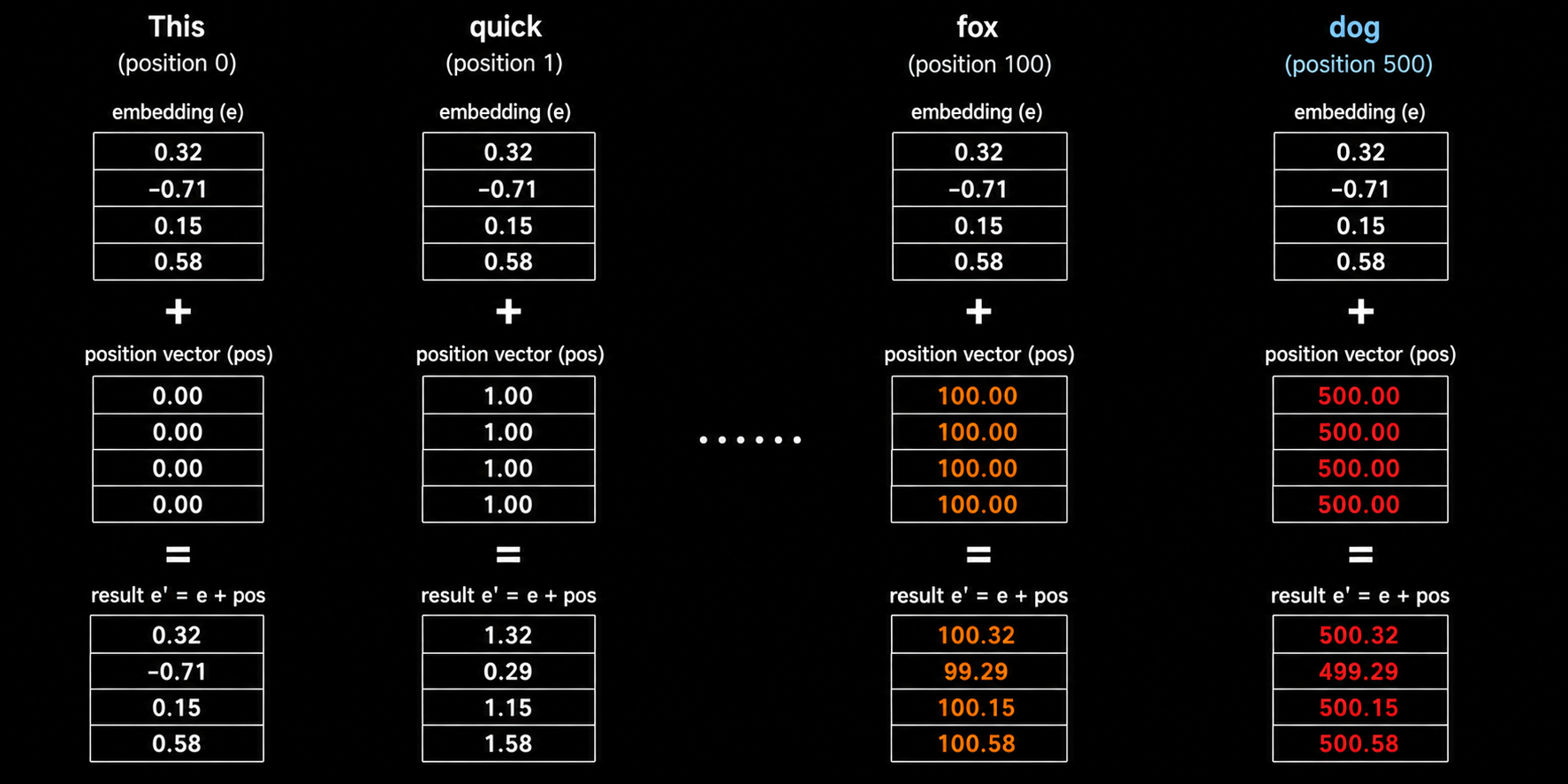
Every token embedding is a vector of numbers, typically around the range of -1 to +1. The proposal is straightforward: take the position index and add it as a scalar to every dimension of the embedding vector.
\[e_i' = e_i + i\]where $i$ is the position of the token in the sequence.
For a sequence “Dog bites man”:
- Position 0: $e_{\text{dog}}’ = e_{\text{dog}} + 0$
- Position 1: $e_{\text{bites}}’ = e_{\text{bites}} + 1$
- Position 2: $e_{\text{man}}’ = e_{\text{man}} + 2$
Now “Dog bites man” and “Man bites dog” produce different embeddings because the same word gets a different number added depending on where it appears.
But we will face an issue with this approach.
The Scale Problem
Embedding values typically live in the range of -1 to +1 (But the range of values can vary relatively to higher number). These are small, carefully learned numbers that encode the meaning of each token.
Now consider what happens at position 500. We add 500 to every dimension of the embedding. A dimension that was 0.3 becomes 500.3. A dimension that was -0.7 becomes 499.3.
The positional number completely dominates the embedding. The semantic content of the token is over shadowed by a massive positional value. The model can barely see embedding of the token.
At position 0, the embedding is untouched. At position 500, the embedding is almost entirely overwritten by the position value. Tokens near the beginning of a sequence and tokens near the end, live in completely different numerical ranges, not only because they mean different things, but also because of where they appear.

No Upper Bound
This approach has no fixed range. The position value grows without limit as the sequence gets longer.
A model trained on sequences of length 512 has seen position values from 0 to 511 . At inference time, if the input has 1024 tokens, the model suddenly sees position values up to 1023. It has never encountered numbers this large during training.
This is an out of distribution problem. The model has no way to generalize to positions it has never seen.
Inconsistent Distance
The absolute difference between position 1 and position 2 is 1. The absolute difference between position 500 and position 501 is also 1.
But relative to the position values themselves, these gaps are very different.
The model cannot learn a consistent notion of “subsequent positions” because the same gap of absolute positional difference of 1 looks completely different depending on where in the sequence it occurs.
Three issues make raw integer positions unusable:
- Scale mismatch. Large position values dominate out the semantic content of embeddings. A token’s meaning becomes invisible behind its position number.
- No upper bound. Position values grow without limit. The model cannot generalize to sequence lengths it has not seen during training.
- Inconsistent distances. The same gap between two positions looks different depending on absolute position. The model cannot learn a uniform sense of distance.
The position values are unbounded and live on a completely different scale than the embeddings.
What if we fix the scale problem by forcing all position values into a fixed range?.
Idea 2: Normalized Positions
Raw integer positions failed because the values were too large. They overwhelmed the embeddings and had no upper bound.
Instead can we just: squeeze all position values into the range [0, 1].
The Idea
Divide each position by the length of the sequence minus one.
\[PE(pos) = \frac{pos}{L - 1}\]where $L$ is the total number of tokens in the sequence.
For a sequence of length 512:
- Position 0 → 0.0
- Position 255 → 0.5
- Position 511 → 1.0
Every position now maps to a value between 0 and 1. No matter how long the sequence is, the values never exceed 1. They sit comfortably in the same range as the embedding values.
The scale problem is gone. The model no longer has to deal with position values like 500 drowning out embedding values like 0.3.
So this works?
The Spacing Problem
Consider two sequences of different lengths.
A short sequence with 10 tokens:
\[[0.0,\ 0.11,\ 0.22,\ 0.33,\ 0.44,\ 0.56,\ 0.67,\ 0.78,\ 0.89,\ 1.0]\]The spacing between consecutive positions is 0.11.
A long sequence with 1000 tokens:
\[[0.0,\ 0.001,\ 0.002,\ 0.003,\ \dots,\ 0.999,\ 1.0]\]The spacing between consecutive positions is 0.001.
The gap between adjacent tokens is 100 times smaller in the long sequence than in the short sequence. Two tokens that are “one step apart” look very different to the model depending on sequence length.
Same Position, Different Values
The same position index maps to completely different values depending on the sequence length.
Position 5 in a 10 token sequence:
\[PE(5) = \frac{5}{9} = 0.556\]Position 5 in a 1000 token sequence:
\[PE(5) = \frac{5}{999} = 0.005\]The fifth token gets the value 0.556 in one case and 0.005 in the other. These are not even close.
The model cannot learn what “position 5” means because the value it receives changes with every input. A model trained mostly on short sequences will associate 0.5 with the middle of a sentence. When it sees a long sequence where 0.5 maps to position 500, the learned association breaks.
Why This Is Fundamental
The root cause is that this scheme is relative to sequence length. It does not encode absolute position. It encodes “how far through the sequence are we.”
Position 0 always means “beginning.” Position 1.0 always means “end.” But everything in between shifts depending on $L$.
This creates two failures:
- No consistent position identity. The same position index produces different values for different sequence lengths. The model cannot learn a stable representation for any position.
- No consistent spacing. The distance between consecutive positions depends on $L$. The model cannot learn a uniform notion of “adjacent tokens” because the numerical gap changes per sequence.
What We Need Instead
Both attempts so far used a single number to represent each position. The first attempt used numbers that were too large. The second attempt used numbers that changed meaning depending on context length.
What if instead of a single number, we represented each position as a vector? And what if that vector used a fixed, length independent pattern that gave every position a unique and consistent representation?
This is exactly what binary encoding do.
Idea 3: Binary Encoding
Both previous approaches used a single number to represent each position. That single number was either too large or too unstable across sequence lengths.
A different idea: represent each position as a vector of bits.
Positions as Binary Vectors
Every integer can be written in binary. We can use this binary representation directly as a position encoding vector.
For a 9 bit encoding:
| Position | Binary Vector |
|---|---|
| 0 | [0, 0, 0, 0, 0, 0, 0, 0, 0] |
| 1 | [0, 0, 0, 0, 0, 0, 0, 0, 1] |
| 2 | [0, 0, 0, 0, 0, 0, 0, 1, 0] |
| 5 | [0, 0, 0, 0, 0, 0, 1, 0, 1] |
| 255 | [0, 1, 1, 1, 1, 1, 1, 1, 1] |
| 511 | [1, 1, 1, 1, 1, 1, 1, 1, 1] |
Each position gets a unique vector of 0s and 1s. The dimensionality of the vector is $\lceil \log_2(L) \rceil$, where $L$ is the maximum sequence length. For a sequence of up to 512 tokens, we need 9 bits.
What Binary Encoding Gets Right
This approach fixes every problem from the previous two attempts.
Bounded values. Every entry in the vector is either 0 or 1. No position value ever exceeds 1. There is no risk of drowning out the embedding.
Unique per position. Every integer has a distinct binary representation. No two positions share the same vector. Position 5 is always [0, 0, 0, 0, 0, 0, 1, 0, 1], regardless of how long the sequence is.
Length independent. Unlike normalized positions, the encoding of position 5 does not change when the sequence length changes. Position 5 is the same vector whether the sequence has 10 tokens or 10,000 tokens.
Fixed dimensionality. The encoding uses $\lceil \log_2(L) \rceil$ dimensions. This grows very slowly. 10 bits can handle sequences up to 1024. 20 bits can handle sequences up to 1,048,576.
But something interesting is hidden in how these bits change across positions. Before we look at the problems, let us first look at the structure.
The Frequency Pattern in Binary
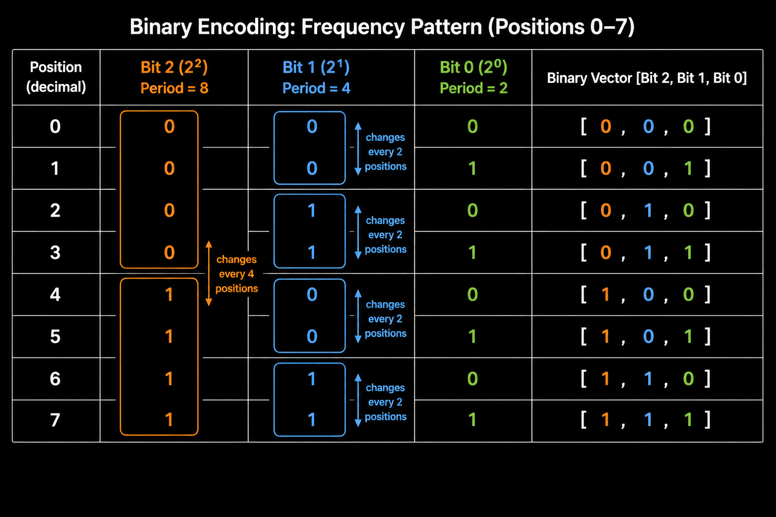
The binary representations for positions 0 through 7 is as below and if we look at each bit column separately.
| Position | Bit 2 ($2^2$) | Bit 1 ($2^1$) | Bit 0 ($2^0$) |
|---|---|---|---|
| 0 | 0 | 0 | 0 |
| 1 | 0 | 0 | 1 |
| 2 | 0 | 1 | 0 |
| 3 | 0 | 1 | 1 |
| 4 | 1 | 0 | 0 |
| 5 | 1 | 0 | 1 |
| 6 | 1 | 1 | 0 |
| 7 | 1 | 1 | 1 |
Now read each column from top to bottom.
Bit 0 (the rightmost, least significant bit) flips every single position: 0, 1, 0, 1, 0, 1, 0, 1. It completes a full cycle every 2 positions.
Bit 1 flips every 2 positions: 0, 0, 1, 1, 0, 0, 1, 1. It completes a full cycle every 4 positions.
Bit 2 flips every 4 positions: 0, 0, 0, 0, 1, 1, 1, 1. It completes a full cycle every 8 positions.
The frequency of that wave depends on which bit position it is.
LSB vs MSB: Fast Bits and Slow Bits
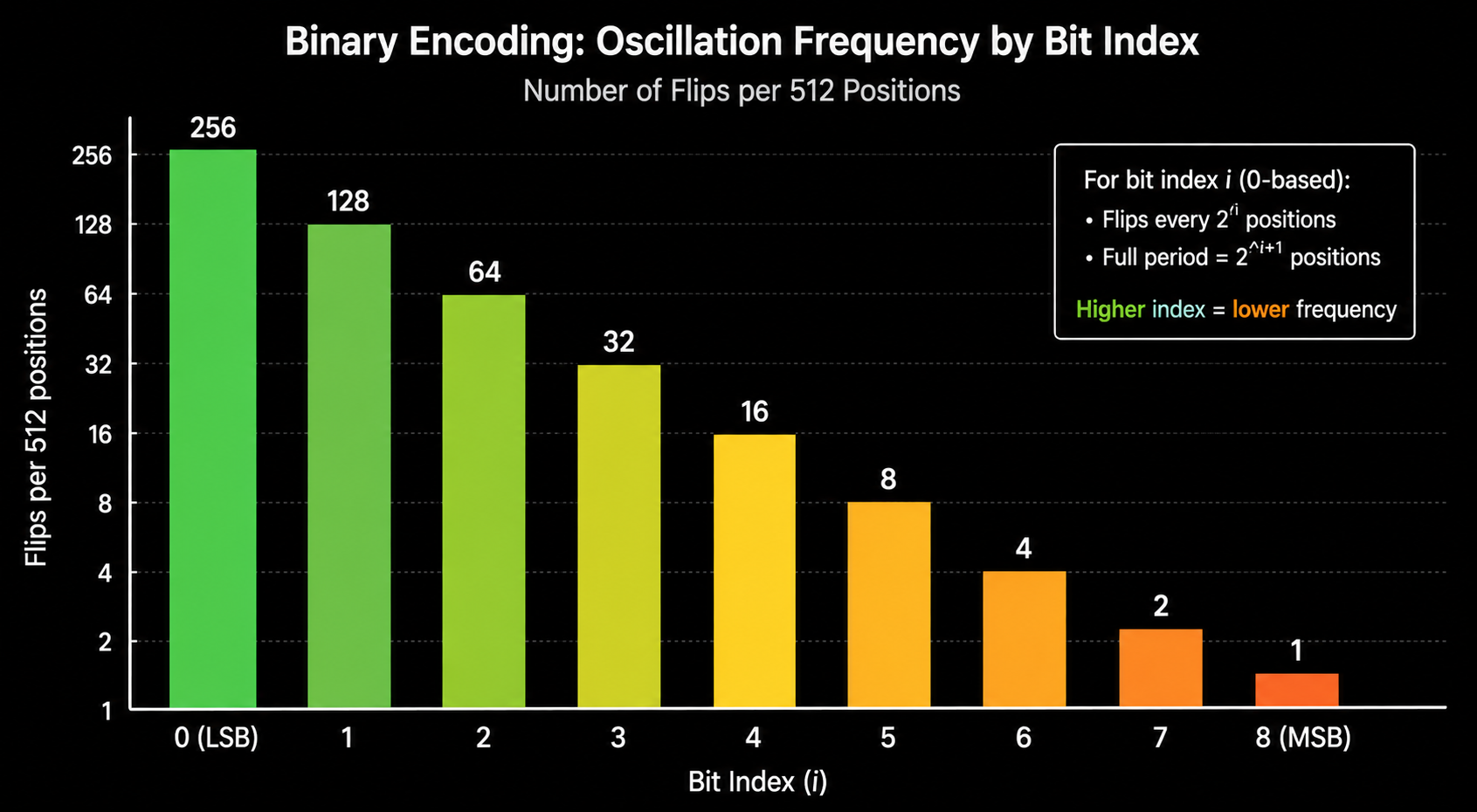
This pattern generalizes to any number of bits. For bit position $i$ (counting from the right, starting at 0):
\[\text{Oscillation period of bit } i = 2^{i+1} \text{ positions}\]The least significant bit (LSB, rightmost, $i = 0$) oscillates the fastest. It flips at every single position. It has a period of 2.
The most significant bit (MSB, leftmost, $i = d-1$) oscillates the slowest. For a 9 bit encoding, it flips every 256 positions. It has a period of 512.
Bits on the right change rapidly. Bits on the left change slowly. Each bit position captures positional information at a different scale.
| Bit Position | Flips Every | Period | Role |
|---|---|---|---|
| Bit 0 (LSB) | 1 position | 2 | Finest grain, changes constantly |
| Bit 1 | 2 positions | 4 | |
| Bit 2 | 4 positions | 8 | |
| Bit 3 | 8 positions | 16 | |
| … | … | … | |
| Bit 8 (MSB) | 256 positions | 512 | Coarsest grain, barely changes |
Visualizing the Square Waves
If you plot the value of each bit across all positions, you see a series of square waves stacked on top of each other. Each wave has exactly half the frequency of the one below it.
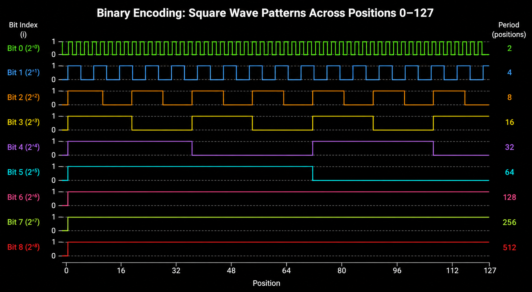
This is a multi frequency encoding. The lowest bit gives fine grained position information (is this an even or odd position?). The highest bit gives coarse position information (are we in the first half or second half of the sequence?).
This multi frequency structure is the most important observation about binary encoding. It will directly motivate sinusoidal positional encoding in the next subsequent blog.
The Discontinuity Problem
Despite this awesome frequency structure, binary encoding has a flaw.
Look at positions 3 and 4:
- Position 3: [0, 1, 1]
- Position 4: [1, 0, 0]
These two positions are adjacent. They are one step apart. But their binary vectors differ in all three bits. The distance between them in vector space is large.
Now look at positions 2 and 3:
- Position 2: [0, 1, 0]
- Position 3: [0, 1, 1]
Also adjacent. Also one step apart. But only one bit differs. The distance between them is small.

Adjacent positions have wildly inconsistent distances in the encoding space. The transition from 3 to 4 is a large jump. The transition from 2 to 3 is a tiny step. There is no smooth relationship between position and encoding.
This happens because binary numbers carry over. When all lower bits are 1, the next increment flips them all to 0 and flips the next higher bit to 1. These carry overs cause sudden large changes in the vector for what should be a small step in position.
Why Discontinuity Matters
Neural networks learn smooth functions. They work best when small changes in input produce small changes in output. If two positions are close together, their encodings should also be close together.
Binary encoding violates this. The model cannot learn a smooth notion of “nearby positions” because the encoding jumps unpredictably between adjacent positions.
What We Keep, What We Fix
Binary encoding gave us two valuable ideas:
- Multi frequency structure. Different bits capture position at different scales. Fast bits for fine detail, slow bits for coarse structure.
- Vector representation. Each position is a vector, not a single number.
But it also has one critical issue:
- Discrete jumps. The square wave transitions between 0 and 1 are discontinuous. Adjacent positions can have very different encodings.
The fix is can be simple. Replace the square waves with smooth waves. Replace the discrete 0/1 flips with continuous sine and cosine functions.
Keep the multi frequency structure. Make it smooth.
This is exactly what sinusoidal positional encoding does.Lets discuss about this in subsequent next blog!
Part 2 of this series covers sinusoidal positional encoding and Rotary Position Embeddings (RoPE) the method used in nearly every modern large language model including LLaMA, Mistral, and Gemma.
References
-
Vaswani, A., Shazeer, N., Parmar, N., Uszkoreit, J., Jones, L., Gomez, A. N., Kaiser, L., Polosukhin, I. (2017). Attention Is All You Need. arXiv:1706.03762
-
Su, J., Lu, Y., Pan, S., Murtadha, A., Wen, B., Liu, Y. (2021). RoFormer: Enhanced Transformer with Rotary Position Embedding. arXiv:2104.09864
-
Biderman, S., Black, S., Foster, C., Gao, L., Hallahan, E., He, H., Wang, B., Wang, P. (2021). Rotary Embeddings: A Relative Revolution. EleutherAI Blog. blog.eleuther.ai/rotary-embeddings
-
Fleetwood. You could have designed state of the art positional encoding. fleetwood.dev/posts/you-could-have-designed-SOTA-positional-encoding